
mc_fit_plot
mc_fit_plot provides visualization and interpretation of the results
generated by mc_fit. The program links the central model analysis
and perturbation analysis by using the perturbation results to estimate
the data uncertainty and misfit imprecision, and then using the
misfit imprecision to identify the central models retained for estimating
aleatoric uncertainty.
mc_fit_plot is available
as both a MATLAB script and a standalone Windows program. The script version
provides more flexibility and is recommended if MATLAB is available. The
switches and parameters controlling the MATLAB plotting scripts are summarized
in mc_fit_plot options.
The description below assumes that the best central model has been
chosen by minimizing misfit. If the best central model has been chosen
to maximize the Bayes score, the same procedure applies, except that
ln(Bayes) replaces ln(misfit), larger objective-function values are
better, and the bad tail of the perturbation distribution is the low-value tail.
Hint
MATLAB sometimes has difficulties arranging figure panels. To avoid these,
maximize the MATLAB figure window before selecting the
my_project_perturbed.pts file.
Standard workflow
The standard mc_fit_plot workflow reads a pair of files generated by
mc_fit: my_project_perturbed.pts and my_project_central.pts. The
user selects the perturbation file; the corresponding central file is then read
automatically.
Warning
mc_fit_plot throws an error if the my_project_perturbed.pts contains
no successful perturbation results. Use one of the auxiliary plotting scripts to inspect a my_project_central.pts file
without this constraint.
Select the
my_project_perturbed.ptsfile of interest.Select two inversion parameters of interest, usually pressure and temperature.
mc_fit_plotautomatically selectsln(misfit)orln(Bayes)as the third plotted variable.If the perturbation results include both models that do and models that do not satisfy the fit-all-data criterion,
mc_fit_plotasks whether to retain only fitting perturbation models. If this filter is accepted, the same fit-based filter is applied to the central models. If it is declined, the user is asked separately whether to apply the fit-based filter to the central models. No prompt appears if all or none of the models satisfy the criterion.The perturbation results are plotted first. These provide the data uncertainty and misfit imprecision. If outlier_filter [default:
true] is enabled, objective-function outliers are removed before the imprecision and uncertainty statistics are estimated.The central results are then plotted. If filter [default:
true] is enabled, central models are filtered by the imprecision interval determined from the perturbation analysis. The retained central models characterize the aleatoric uncertainty of the inverse solution.The perturbation panel is automatically redrawn after the central model analysis is finalized so that the best-central marker, legend entry, uncertainty graphics, and covariance ellipse are all centered on the final best central model. This matters if application of the fit-all-data criterion changes which central model is identified as best.
The figure is exported automatically. By default, the output is a bitmap
.pngfile. If outPDF [default:false] is enabled, the output is a vector.pdffile.
The standard figure
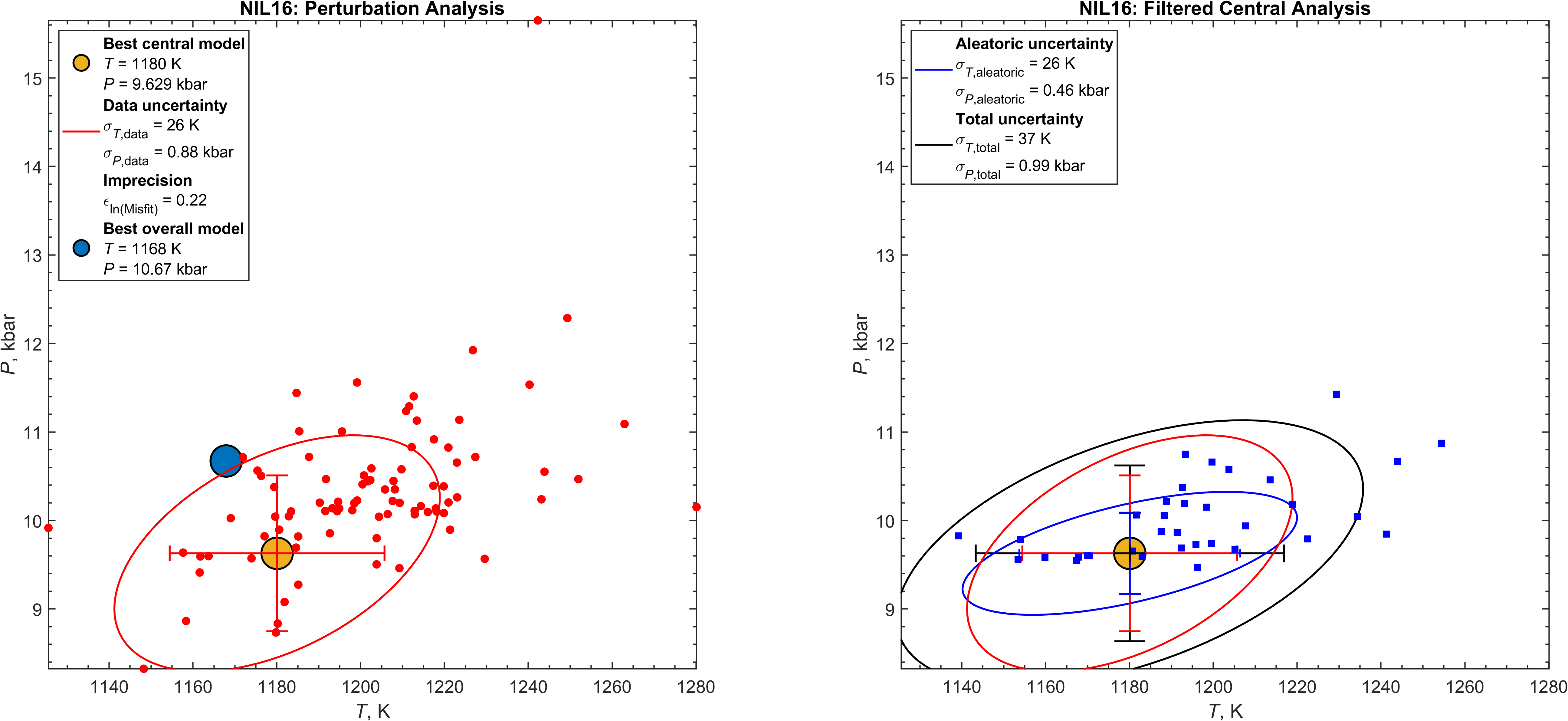
The standard figure generated by mc_fit_plot summarizes the two stages of
the analysis (Fig. 4). The left panel summarizes the
perturbation analysis; the right panel summarizes the
central model analysis after application of the perturbation-derived
imprecision filter.
The following sections describe the main graphical elements in the standard figure. References to plotting options are included where they are relevant to the discussion. The complete option reference is given in mc_fit_plot options.
—
Perturbation analysis panel
The left panel of the standard figure shows the perturbation results. The small red symbols are the optimized models obtained after randomly perturbing the analytical and thermodynamic data within their uncertainties. Because every perturbation optimization begins from the best central model, the scatter of these results estimates the data uncertainty.
The large gold symbol marks the best central model.
The perturbation-derived error bars and covariance ellipse are centered on this point.
They represent the data uncertainty. Their probability coverage is controlled by sigma_level [default: 1]. By default, they correspond to approximately 68% probability coverage.
The scatter of the transformed objective-function values in the perturbation analysis estimates the misfit imprecision, \(\epsilon_{\ln(\mathrm{misfit})}\). This quantity is reported in the left-panel legend and is used to define the imprecision interval applied to the central models in the right panel.
If a perturbed optimization has a lower misfit than the best central model, the best-fitting perturbation result is identified as the best overall model. In Fig. 4, this model is shown by the large blue symbol in the left panel. The best overall model remains part of the perturbation ensemble used to estimate data uncertainty; identifying it separately is diagnostic. In most cases it simply reflects the expected spread of objective-function values generated by perturbing the analytical and thermodynamic data. However, if the best overall model lies well outside the imprecision interval of the best central model or has a substantially lower objective-function value, it may be worthwhile to examine the perturbation that produced it to determine whether a particular analytical or thermodynamic perturbation has an unusually large influence on the inversion. Display of the marker is controlled by plotbst.
—
Central model analysis panel
The right panel of Fig. 4 shows the central models retained after applying the imprecision interval determined from the perturbation analysis. These models were obtained with the analytical and thermodynamic data fixed at their central values. Their scatter characterizes the aleatoric uncertainty of the inverse solution.
The small square symbols in the right panel are the retained central models. The large gold symbol again marks the best central model. The blue error bars and blue covariance ellipse represent the aleatoric component estimated from the retained central models. The black error bars and black covariance ellipse represent the total uncertainty, obtained by combining the data and aleatoric covariance matrices in quadrature, assuming that these two sources are independent.
Central-model filtering is controlled by filter. With the default
setting, only central models within the perturbation-derived imprecision
interval of the best central model are retained for estimating aleatoric
uncertainty.
The probability coverage of the imprecision interval and the uncertainty bars
and covariance ellipses is controlled by sigma_level
[default: 1], corresponding to approximately 68% coverage.
—
Marker filling and the fit-all-data criterion
Marker filling indicates the result of the fit-all-data criterion, not membership in the imprecision interval. By default, auto_filled_symbols_for_nofit lets the script choose the marker-fill convention from the distribution of fitting and non-fitting models. The convention can be fixed manually with filled_symbols_for_nofit.
The fit-all-data criterion is independent of the imprecision-based filtering used to estimate aleatoric uncertainty. It can be useful for identifying models that satisfy all individual observations within their assigned uncertainties, but it should not be confused with the perturbation-derived imprecision filter.
—
Legends
The legends in the two panels of the standard figure are complementary rather than redundant. The left-panel legend identifies the best central model, reports the data uncertainty, gives the misfit imprecision, and identifies the best overall model when one is present. The right-panel legend reports the aleatoric uncertainty estimated from the retained central models and the total uncertainty obtained by combining the data and aleatoric covariance matrices.
—
Alternative inversion parameters
The standard figure displays two selected inversion parameters, usually
pressure and temperature.
Uncertainties and correlations involving additional
inversion parameters can be evaluated by selecting different parameters from the
mc_fit_plot interface. The same interpretation applies: the perturbation
panel shows the data uncertainty for the selected parameter pair, and the central
panel shows the retained central models and the corresponding aleatoric and
total uncertainty estimates.
Exporting modified figures
mc_fit_plot exports the generated figure automatically. If the figure is
modified after the script finishes, new .png and .pdf files can be
generated from MATLAB with, for example:
% Export the current figure to my_project.png
exportgraphics(gcf,'my_project.png','ContentType','image','Resolution',300);
% Export the current figure to my_project.pdf
exportgraphics(gcf,'my_project.pdf','ContentType','vector','BackgroundColor','none');
Filtering and diagnostics
Several filters can affect the plotted results, but only the
imprecision filter is fundamental to the uncertainty strategy
used by mc_fit_plot. The perturbation-derived misfit imprecision
determines which central models are retained and therefore controls the
estimate of aleatoric uncertainty.
Other filters are diagnostic or practical. The fit-all-data filter uses the assigned analytical uncertainties to classify or optionally retain models that satisfy all observations. Objective-function outlier filtering removes anomalous perturbation results before imprecision and covariance are estimated.
Auxiliary visualization scripts
Several MATLAB scripts for generating alternative mc_fit data visualizations are available. These use the same functions and option <mc_fit_plot_options>` structure as mc_fit_plot.
—
mc_fit_data_uncertainty_components_plot
Plots the thermodynamic and analytical components of the
data uncertainty together with the resulting total data uncertainty
(e.g. Fig. 10 or Fig. 7). This plot is useful for
visualizing the relative contributions of the two uncertainty components and
how they combine to produce the total data uncertainty. This script requires that the user select a consistent pair of
*_perturbed.pts files.
—
mc_fit_imprecision_band_plot
Plots the perturbation and central results in either the
\(x\)–ln(misfit) or \(y\)–ln(misfit) projection and shades
the imprecision interval (e.g. Fig. 9 or Fig. 6). This visualization is useful for understanding how
the perturbation-derived misfit imprecision selects the retained central
models.
—
mc_fit_plot_legacy
Reproduces the pre-7.2.6 mc_fit_plot output and workflow. The legacy script requires a consistent pair of *_central.pts and *_perturbed.pts files.
mc_fit_multi_plot
Builds a combined figure from multiple selected *.pts files. It can link
X and Y axes across panels. This script can be used to inspect any choice of
input files.
—
mc_fit_permutation_plot
Does the standard mc_fit_plot analysis for multiple inversion
problems and superimposes the best central models and uncertainty ellipses. The resulting three-panel figure compares the
data, aleatoric, and total uncertainty of the selected problems. This script
is useful for evaluating the effects of alternative data
(Fig. 16) or model (Fig. 19)
permutations on the preferred solution and its uncertainty.
—
mc_fit_single_plot
Plots a single *.pts file. This script is useful for inspecting either a
central or perturbation file independently and preserves manual filtering
dialogs by default.
See also mc_fit_multi_plot and mc_fit_triple_plot.
—
mc_fit_triple_plot
Produces a three-panel view consisting of a large X-Y panel and
smaller X-Z and Y-Z panels. This script can be used to inspect any
mc_fit *.pts file.
