
Examples
This section is a guide to the mc_fit example input/output files
in the examples directory. The examples are structured so that, aside from introductory text, the scientific narrative is largely provided within extended captions for the figures generated by the mc_fit_plot MATLAB scripts. The remaining text summarizes the quantitative details of each inversion problem and its resolution.
mc_fit problems can be broadly categorized as:
Bulk-equilibrium problems constrained by a measured bulk composition.
Bulk-equilibrium problems constrained by measured phase proportions.
Bulk-equilibrium problems without bulk composition and modal constraints.
The first category is by far the least costly. The cost of the remaining categories rises rapidly with the number of observed phases. Since any subset of equilibrium phases is also at equilibrium, it is wise, when treating problems of these latter categories, to begin with a subset of the observed phases that unambiguously represents a relict equilibrium and then to progressively add additional phases. If the addition of a phase causes the problem to become intractable, then either the phase was not part of the relict equilibrium, or the thermodynamic model for the assemblage is flawed. The resolution of such issues is petrology.
Local-equilibrium problems with no unique bulk composition
This category corresponds most closely to classical thermobarometry. Its only assumption is that a selected set of observed phases record the compositions of an equilibrium at the time of interest. It is most appropriate for polymetamorphic rocks and/or rocks with zoned minerals.
—
bl_Chi: A synthetic garnet-clinopyroxene problem
This is a synthetic problem with a known solution designed to test mc_fit.
Fig. 5 is the The standard figure of the inversion results, while
Fig. 6 and Fig. 7
provide additional detail by illustrating how the misfit scatter is used to estimate
aleatoric uncertainty and by separating the analytical and thermodynamic components
of the inversion parameter uncertainties.
The problem was created by:
Computing phase equilibria for a metabasaltic composition in the system Na2O-CaO-K2O-FeO-MgO-Al2O3-TiO2-SiO2-H2O-O2 at T = 1000 K and P = 10 kbar using the Perple_X program
meemum(bl478.dat).The compositions of coexisting clinopyroxene and garnet were extracted from the
meemumforward model (bl478.prn).The excess oxygen component was stripped from the garnet and clinopyroxene compositions, making O2 an unmeasured component in the inverse problem. Additionally, the forward components not present in the garnet and clinopyroxene models (K2O, TiO2, H2O) were eliminated from the original input (bl_Chi.dat).
To make the test challenging, the ranges for pressure, temperature, and the unmeasured O2 component were set so that their centroid was far from the known solution (bl_Chi.imc).
Additional details:
I/O files: examples/bl_Chi
Chemical system ([Green2016], bl_Chi.dat): Na2O-CaO-FeO-MgO-Al2O3-SiO2-O2
Saturated components: None
Unmeasured component: O2
Data uncertainties:
Analytical: simulated with a reciprocal function similar to Eq 8 (bl_Chi.imc). In the current version of
mc_fit, this simulation is automatic if an uncertainty is assigned a negative value.Thermodynamic: [Green2016], (hp62ver.dat).
Modified Perple_X options (perplex_option.dat): None
Modified
mc_fitoptions (bl_Chi_MC_fit_option.dat):number_of_tries increased to
250to ensure adequate sampling of the solution space.
Modified
mc_fit_plotoptions:convert_to_C set to
Fto display temperatures in Kelvin.
Best central model:
\(P\) = 10.076 kbar
\(T\) = 1001.62 K
\(C_\text{O2}\) = 0.208853
Uncertainty (Fig. 5):
Unmeasured components (Eq 28):
\(\text{molar} \left( \frac{\text{Fe}^{3+}}{\text{Fe}^{2+}} \right)_\text{Cpx}\) = 0.0136
\(\text{molar} \left( \frac{\text{Fe}^{3+}}{\text{Fe}^{2+}} \right)_\text{Grt}\) = 0.00816
Dependent variables, Oxygen fugacity and Delta QFM (Appendix C):
\(\mu_{\text{O2}}\) = -442340 J/mol
\(\log f_{\text{O2}}\) = -14.72 (bar)
\(\Delta_{\text{QFM}}\) = 0.5842
Bulk composition (Appendix B):
Because this problem employs neither bulk compositional nor modal constraints, the best central model bulk composition is not an appropriate forward model for the synthetic source rock (bl478.prn). Nonetheless, the model bulk composition can be used to calculate phase equilibria (cf. Fig. 8) with
meemumorvertexto verify themc_fitprediction and to graphically assess the quality of the prediction with tools such asLinaForma([Mackay2024]),IntersecT([Nerone2025]), and/orwerami.
The examples/bl_Chi/variants subdirectory includes input files for calculations that explore the use of alternative misfit functions (
LSQ,wChi), Bayes score, and the influence of the compositional weighting factor for the misfit function.
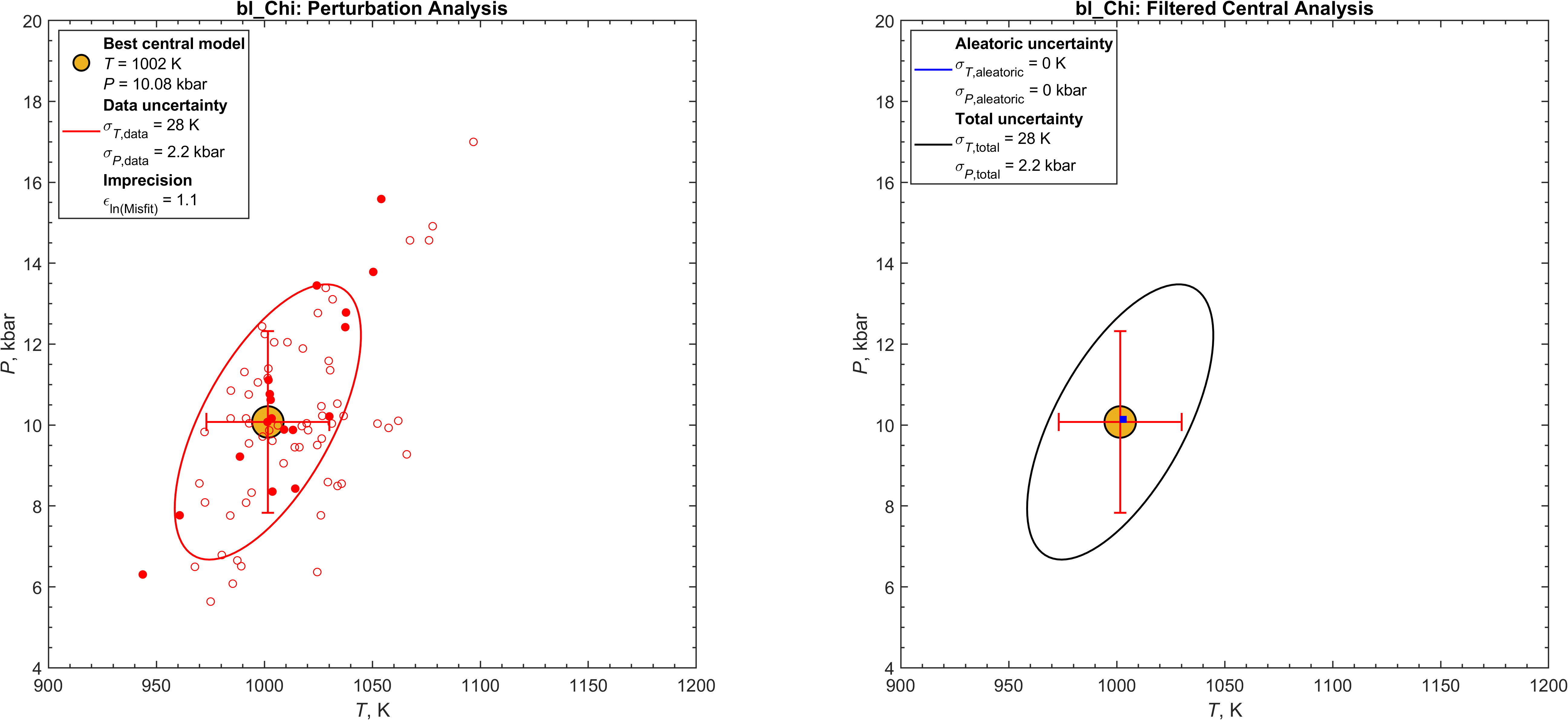
Fig. 5 The bl_Chi synthetic garnet + clinopyroxene problem with a known solution at {P = 10 kbar, T = 1000 K}. Filled symbols represent models that meet the fit-all-data criterion for the analytical data. The fit-all-data filter was not applied because the analytical uncertainties were simulated. Uncertainty intervals and ellipses show the default 68% coverage (sigma_level).
Left panel: Perturbation analysis. Because all optimizations during the perturbation analysis initiate from the best central model coordinate {P = 10076 bar, T = 1001.6 K}, the scatter of the perturbation results quantifies the inversion parameter uncertainties (\(\sigma_{T,\text{data}}\) and \(\sigma_{P,\text{data}}\)) arising from analytical and thermodynamic uncertainty.
Right panel: Filtered central model analysis. Central model results filtered to exclude models outside the imprecision interval of the best central model. Only 2 of the 239 central models lie within the imprecision interval. The low retention rate suggests negligible aleatoric uncertainty, a conclusion supported by the perturbation misfit scatter discussed in Fig. 6.
Uncertainties and correlations for additional inversion parameters, in the present case \(\sigma_{C\text{[O2]}}\), can be evaluated by selecting the parameters from the mc_fit_plot interface.
Generated with mc_fit_plot.
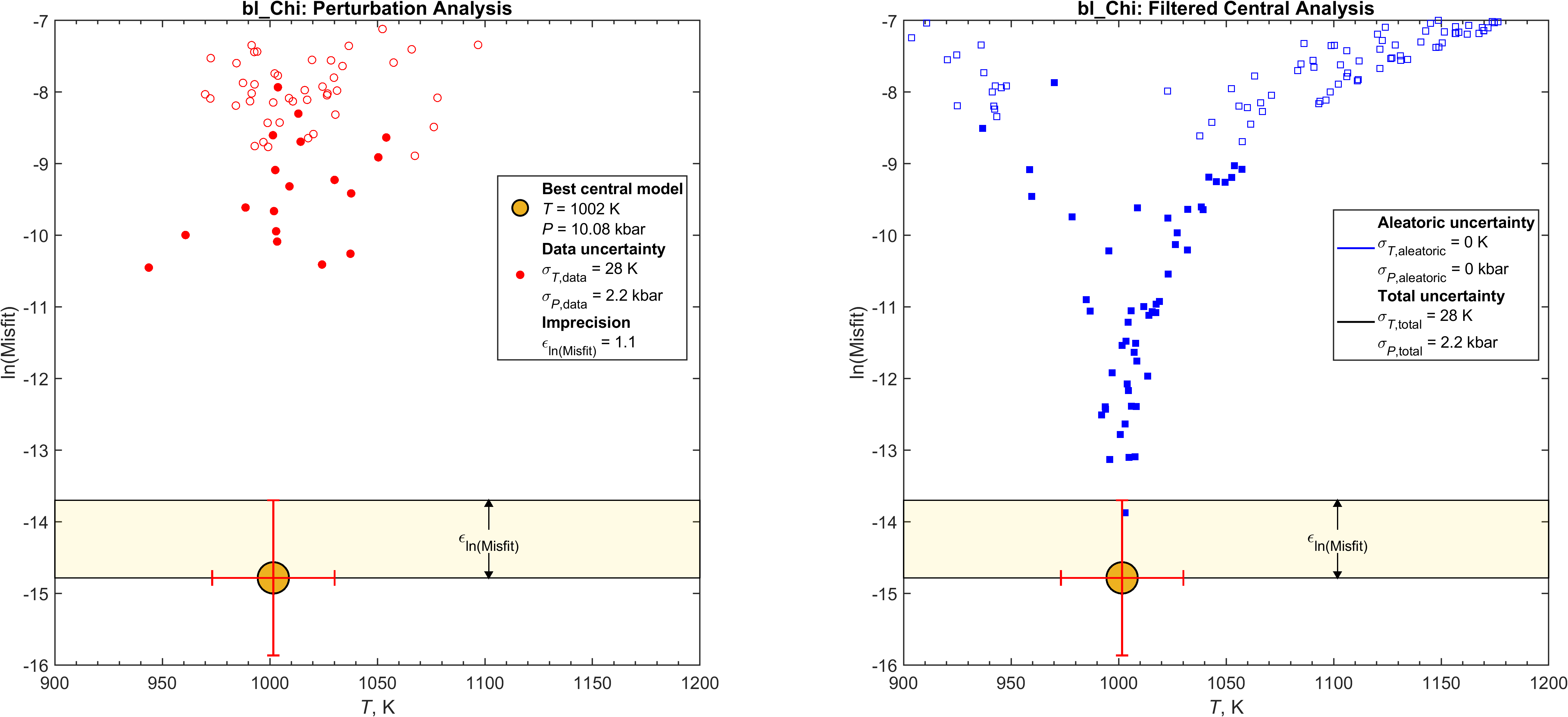
Fig. 6 Figures generated by mc_fit_plot are 3-dimensional plots of two selected inversion parameters and the log of the misfit function of the models output by mc_fit.
By default the plots are displayed in the plane of the selected inversion parameters.
Rotation into an orthogonal plane reveals the misfit scatter, which is essential for understanding how the central models are filtered to estimate the aleatoric uncertainty of the inversion parameters. Here the perturbation analysis and central model misfit scatter are shown in the \(T \text{-} \ln(\text{misfit})\) plane for the bl_Chi inversion.
Left panel: Perturbation analysis misfit scatter. The misfit imprecision (\(\epsilon_{\ln(\text{misfit})}\)) is the standard deviation of the perturbation analysis misfit scatter scaled by sigma_level for the desired coverage. The misfit of the best central model is orders of magnitude smaller than that of the perturbed models and lies far outside the perturbation distribution. This behavior is expected because the synthetic problem was generated using the central values of the analytical and thermodynamic data. Consequently, perturbing these data is expected to increase the misfit. By contrast, in natural problems the central data values are merely estimates of the unknown true values, so perturbations may either increase or decrease the misfit, and the best central model is therefore expected to lie within the perturbation distribution. The yellow band depicts the imprecision interval. The interval is one-sided because the best central model is, by definition, the central model with the lowest misfit.
Right panel: Central model misfit scatter. The standard deviations and covariance of the central model scatter within the imprecision interval are used to estimate the aleatoric uncertainty for the coverage specified by sigma_level. Because only one central model in addition to the best central model lies within the imprecision interval, the sample size is insufficient to estimate standard deviations. Although this circumstance may reflect inadequate sampling of the solution space, the large number of central models and their funnel-shaped distribution, also evident in the \(P \text{-} \ln(\text{misfit})\) plane, suggest that the aleatoric uncertainty is negligible in comparison to the data uncertainty. This interpretation is consistent with the synthetic observations having been generated from an exact solution.
Generated with mc_fit_imprecision_band_plot.
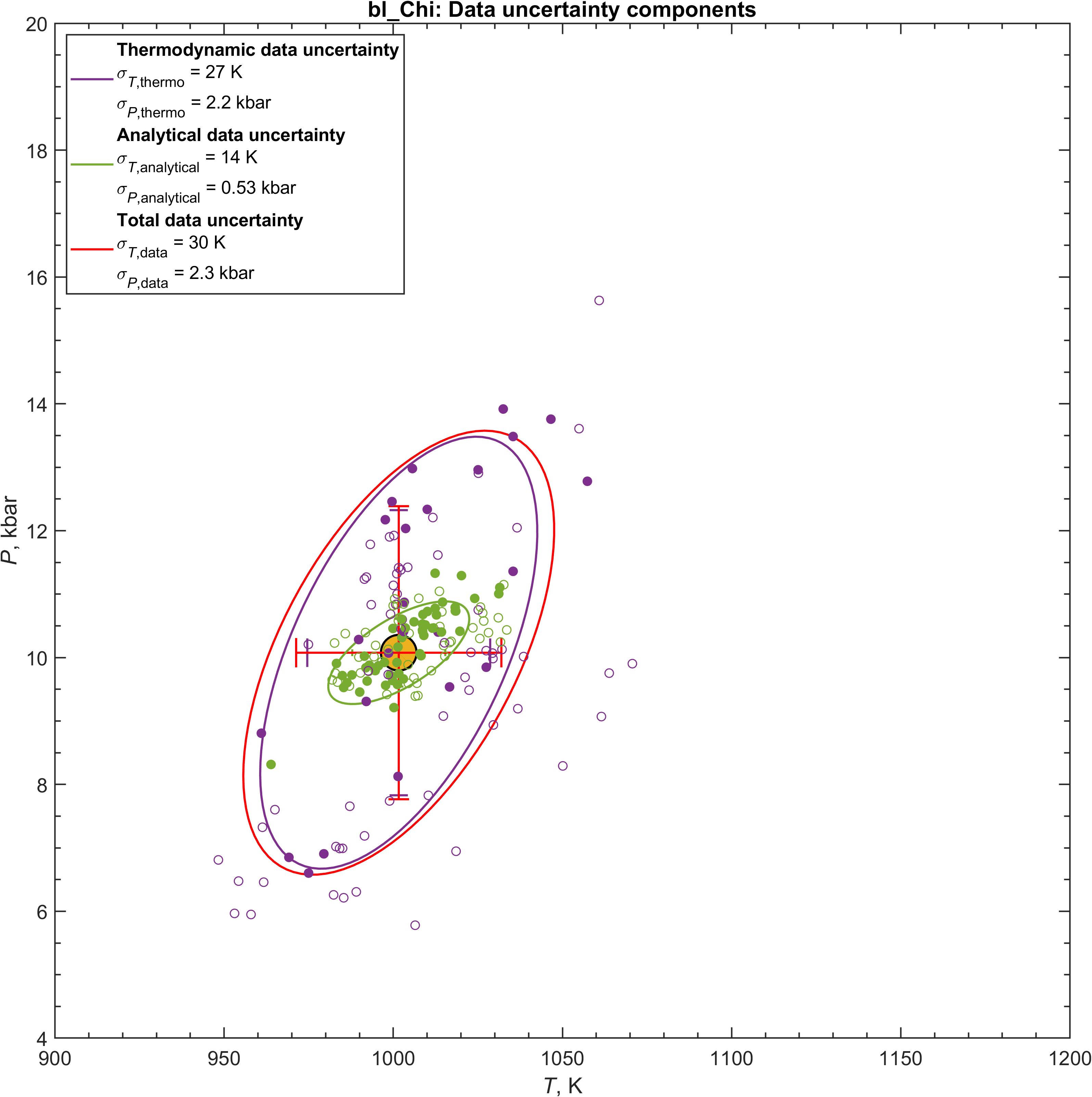
Fig. 7 The thermodynamic and analytical components of the data uncertainty for the bl_Chi inversion. Because the components are estimated from independent perturbation analyses, the total data uncertainty is not numerically identical to that obtained when both sources of error are propagated simultaneously (Fig. 5, left panel).
Increasing the sample size (number_of_perturbations) will cause the two estimates of the total data uncertainty to converge.
The components were computed with mc_fit without repeating the central model analysis by setting the perturbation_hot_start and uncertainties options; the relevant I/O files are at bl_Chi/variants.
Generated with mc_fit_data_uncertainty_components_plot.
—
NIL16: A natural garnet-clinopyroxene problem
This problem treats a natural metagabbro garnet-clinopyroxene assemblage. The sample, NIL16-1,
abbreviated NIL16 hereafter,
is one among a large number of samples from the Nilgiri Block, Southern India, reported and analyzed by
Samuel et al. ([Samuel2019]).
Samuel et al. concluded that the Nilgiri Block was metamorphosed at
P = 7–11 kbar and T = 923–1073 K at relatively oxidizing conditions, 2.5–3 log units above the
fayalite-magnetite-quartz (QFM) buffer.
NIL16 was selected arbitrarily from the samples presented by Samuel et al.
and, for purposes of demonstration, the equilibrium assemblage simplified to include only garnet and
clinopyroxene.
In light of these simplifications, disagreement
between the mc_fit results and those of Samuel et al. should not be construed as criticism of the
latter.
A complete analysis of the NIL16 sample with mc_fit would include the additional phases and/or bulk
compositional constraints provided by Samuel et al.
Fig. 8 is the The standard figure of the inversion results, while Fig. 9 and Fig. 10 provide additional detail by illustrating how the misfit scatter is used to estimate aleatoric uncertainty and by separating the analytical and thermodynamic components of the inversion parameter uncertainties.
—
Additional details:
I/O files: examples/NIL16
Chemical system ([Holland2018], NIL16.dat): Na2O-MgO-Al2O3-TiO2-CaO-Cr2O3-FeO-SiO2-O2
Saturated components: None
Unmeasured component: O2
Data uncertainties:
Analytical ([Samuel2019], NIL16.imc)
Thermodynamic ([Holland2018], hp633ver.dat)
Modified Perple_X options (perplex_option.dat): None.
Modified
mc_fitoptions (NIL16_MC_fit_option.dat):number_of_tries increased to
250to ensure adequate sampling of the solution space.molar_composition_input set to
Fto allow mass fraction input compositions.relative_error set to
Fto make direct use of measured errors.
Best central model
\(P\) = 9629.89 bar
\(T\) = 1180.07 K
\(C_\text{O2}\) = 0.267510
Inversion parameter uncertainties (Fig. 8):
Unmeasured components (Eq 28):
\(\text{molar} \left( \frac{\text{Fe}^{3+}}{\text{Fe}^{2+}} \right)_\text{Cpx}\) = 0.0169
\(\text{molar} \left( \frac{\text{Fe}^{3+}}{\text{Fe}^{2+}} \right)_\text{Grt}\) = 0.00657
Dependent variables, Oxygen fugacity and Delta QFM (Appendix C):
\(\mu_{\text{O2}}\) = -424807 J/mol
\(\log f_{\text{O2}}\) = -11.49 (bar)
\(\Delta_{\text{QFM}}\) = 1.984
This result is consistent with the contention of Samuel et al. ([Samuel2019]) that the Nilgiri Block metagabbros were metamorphosed at oxidized fugacities 2-3 log units above the QFM buffer. In contrast to the
mc_fitresult, deduced entirely from silicates, Samuel et al. estimated \(\Delta_{\text{QFM}}\) from Fe-Ti oxides.
Bulk composition (Appendix B):
Because this problem employs neither bulk compositional nor modal constraints, the best central model bulk composition (Try 128, NIL16.out) is not an appropriate model for the NIL16 rock. Nonetheless, the model bulk composition can be used to calculate phase equilibria (Fig. 8) with
meemumorvertexto verify themc_fitprediction and to graphically assess the quality of the prediction with tools such asLinaForma([Mackay2024]),IntersecT([Nerone2025]), and/orwerami.
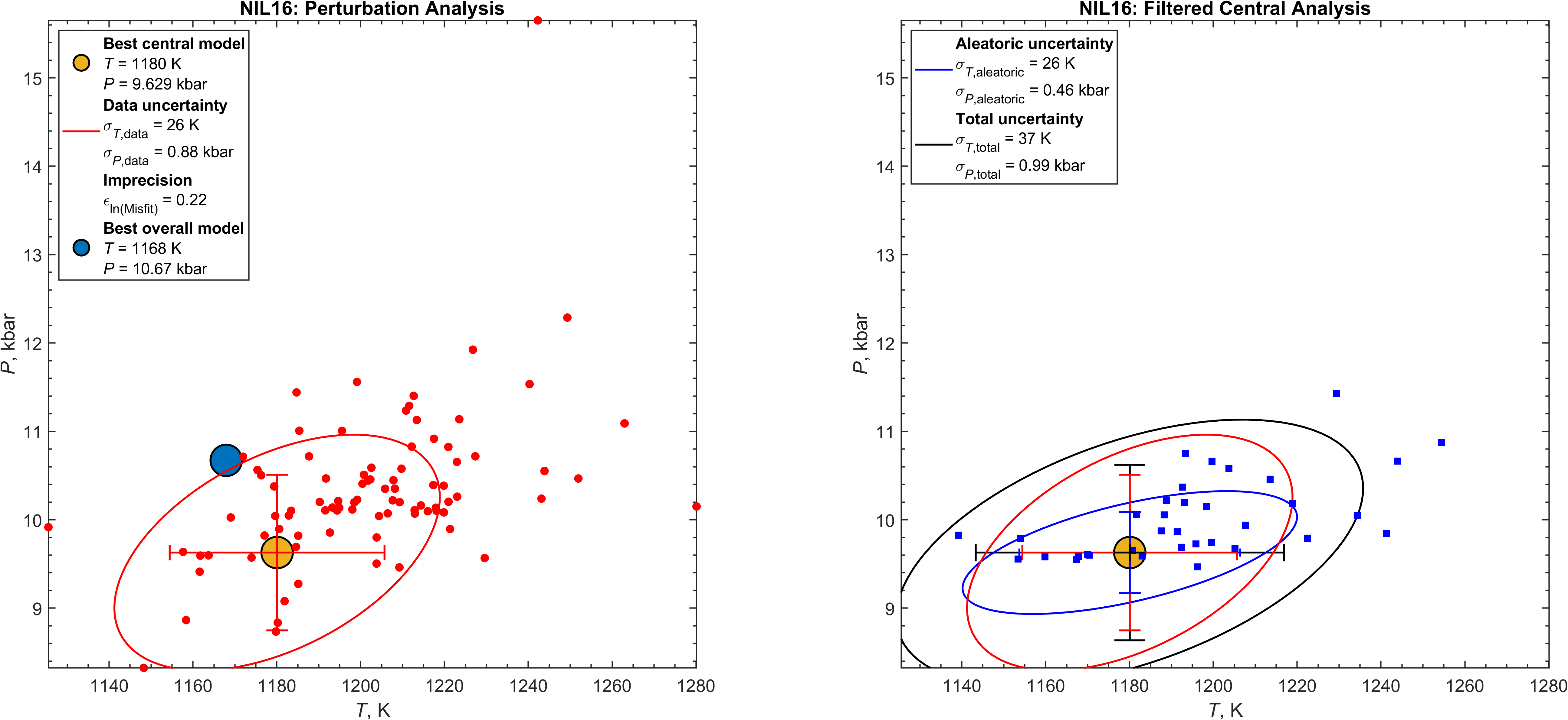
Fig. 8 The NIL16 garnet + clinopyroxene problem.
None of the models satisfy the fit-all-data criterion.
An explanation for this behavior might be that the analytical uncertainties reported by
[Samuel2019] are standard errors of the mean rather than standard
deviations. When either no models or all models satisfy the
fit-all-data criterion, mc_fit_plot uses only filled
symbols by default (auto_filled_symbols_for_nofit).
Uncertainty intervals and
ellipses show the default
68% coverage (sigma_level).
Left panel: Perturbation analysis. Because every optimization during the perturbation analysis is initiated from the best central model (P = 9629 bar, T = 1180 K), the scatter of the perturbation results quantifies the inversion parameter uncertainties (\(\sigma_{T,\text{data}}\) and \(\sigma_{P,\text{data}}\)) arising from analytical and thermodynamic uncertainty. The corresponding misfit scatter, visible in the \(T \text{-} \ln(\text{misfit})\) or \(P \text{-} \ln(\text{misfit})\) plane, is discussed in Fig. 9.
Right panel: Filtered central model analysis.
Central model results filtered to exclude models outside the
imprecision interval of the best central model. In contrast to
the bl_Chi synthetic problem (Fig. 5), a
substantial fraction (36 of 237) of the central models lie within the
imprecision interval. The retained population indicates that the
aleatoric uncertainty is comparable to the
data uncertainty. Total uncertainty intervals and ellipses are
obtained by combining the data and aleatoric uncertainties in
quadrature, assuming the two sources are independent.
Uncertainties and correlations involving additional inversion
parameters, in the present case \(\sigma_{C\text{[O2]}}\), can be
evaluated by selecting the parameters from the mc_fit_plot
interface.
Generated with mc_fit_plot.

Fig. 9 Figures generated by mc_fit_plot are 3-dimensional plots of two selected inversion parameters and the log of the misfit function of the models output by mc_fit.
By default the plots are displayed in the plane of the selected inversion parameters.
Rotation into an orthogonal plane reveals the misfit scatter, which is essential for understanding how the central models are filtered to estimate the aleatoric uncertainty of the inversion parameters. Here the perturbation analysis and central model misfit scatter are shown in the \(T \text{-} \ln(\text{misfit})\) plane for the NIL16 garnet + clinopyroxene problem.
Left panel: Perturbation analysis misfit scatter.
The misfit imprecision (\(\epsilon_{\ln(\text{misfit})}\)) is the standard deviation of the perturbation analysis misfit scatter scaled by sigma_level for the desired coverage.
In contrast to the bl_Chi synthetic problem, the best central model lies within
the perturbation distribution, as expected for a natural problem (compare Fig. 5).
The yellow band depicts the imprecision interval. The interval is one-sided because the best central model is, by definition, the central model with the lowest misfit.
Right panel: Central model misfit scatter.
The standard deviations and covariance of the central model scatter within the imprecision interval are used to estimate the aleatoric uncertainty for the coverage specified by sigma_level.
The misfit of the best central model is comparable to that of the perturbed models. In such cases, it is expected that a perturbation of the best central model may yield a model with lower misfit. When this occurs, mc_fit_plot identifies the perturbed model with the lowest misfit as the best overall model. While the best overall model is a statistically legitimate solution to the thermobarometric problem, for most applications it is not the preferred solution because it implies that the perturbed analytical and thermodynamic data are preferred over the measured and/or published central values. Nonetheless, if the best overall model lies outside the imprecision interval of the best central model, it may be informative to examine the details of the perturbation that produced it to discover whether it has thermodynamic or analytical significance.
Generated with mc_fit_imprecision_band_plot.
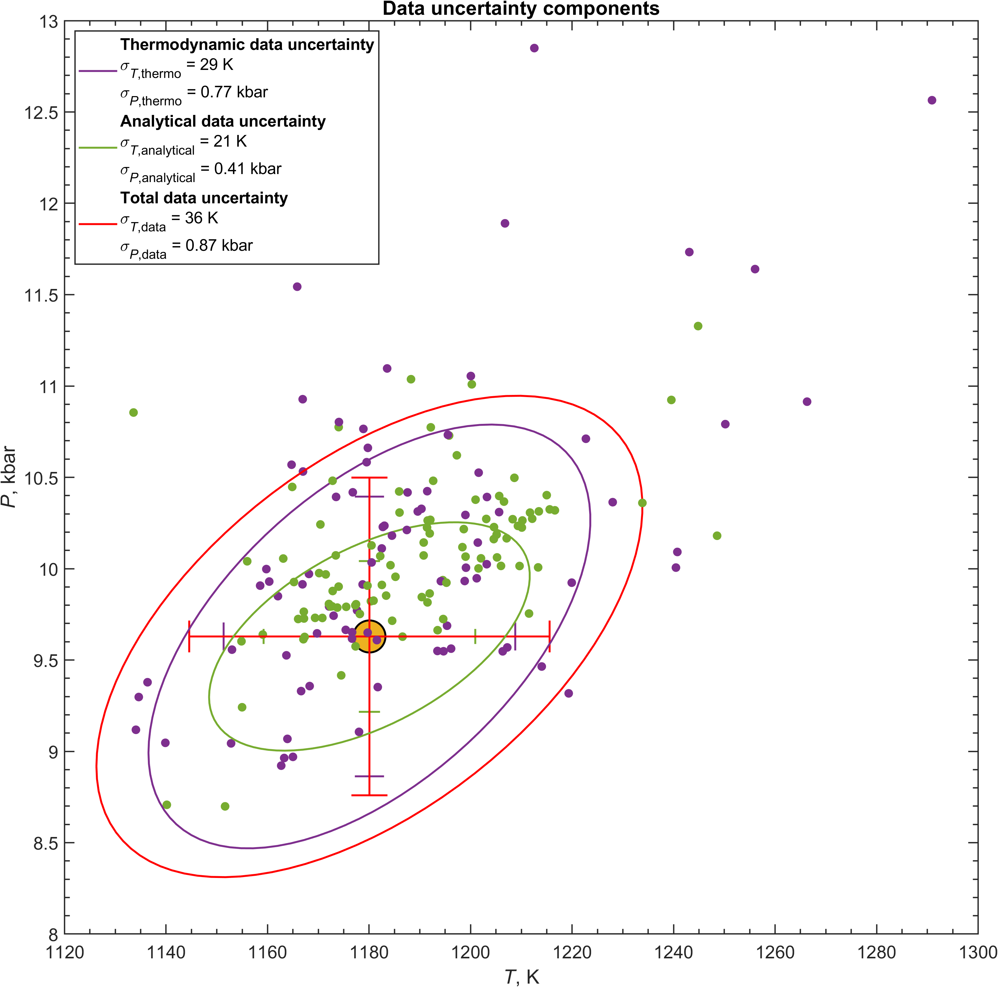
Fig. 10 The thermodynamic and analytical components of the data uncertainty for the NIL16 garnet + clinopyroxene problem. Because the components are estimated from independent perturbation analyses, the total data uncertainty is not numerically identical to that obtained when both sources of error are propagated simultaneously (Fig. 8, left panel).
Increasing the sample size (number_of_perturbations) will cause the two estimates of the total data uncertainty to converge.
The components were computed with mc_fit without repeating the central model analysis by setting the perturbation_hot_start and uncertainties options; the relevant I/O files are at NIL16/uncertainty.
Generated with mc_fit_data_uncertainty_components_plot.
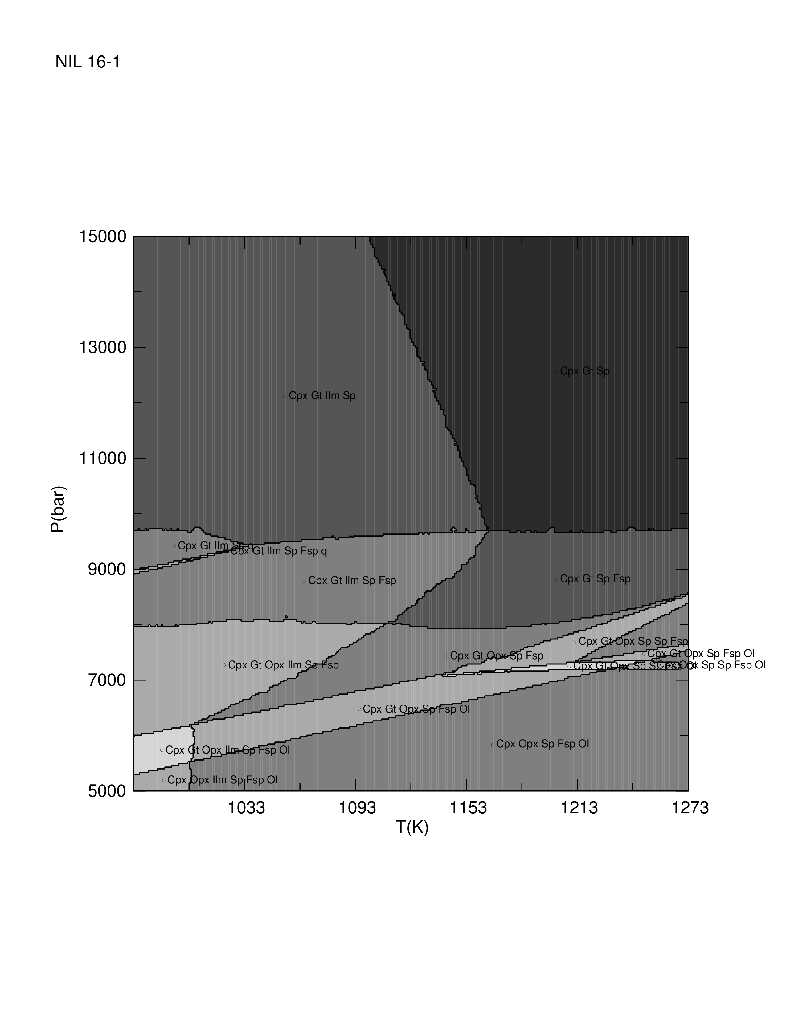
Fig. 11 Calculated P–T phase relations for the best central NIL16 model composition. This
composition is not representative of bulk rock composition (Appendix B).
Bulk-equilibrium problems with bulk compositional constraints
This category is in essence modern thermobarometry. Its key assumptions are:
Existence of a well-defined spatial domain with known bulk chemistry.
The phases within this domain preserve a relict equilibrium.
The emphasis placed on phase diagram sections in modern thermobarometry has created the impression that the bulk composition of a rock is the primary source of thermobarometric information. This impression is mistaken. The observed assemblage identifies the relevant phase field, mineral compositions locate a point within that field, and bulk composition determines the extent of that field. Thermobarometry is concerned only with locating that point; the bulk composition serves only to constrain whether that point is thermodynamically permissible. Put another way, knowledge of the bulk composition is essential for calculating a phase diagram section and for determining whether the inferred equilibrium is thermodynamically permissible, but it is not the source of the thermobarometric information.
The use of bulk in mc_fit compositional constraints has both advantages and disadvantages:
Pro: the constraints reduce the dimension of the inversion problem and thereby speed
mc_fitcalculations.Pro: if the bulk compositional information is incomplete,
mc_fitestimates the missing information by inversion. The completed bulk composition can then be used to calculate a phase diagram section to reconstruct the equilibrium history of the rock. This obviates the usual guessing of unmeasured bulk chemistry that often accompanies the use of phase diagram sections in petrology.Con: bulk compositional constraints require that the complete observed mineralogy must be included in the inversion problem. This requirement precludes the use of subsets of the observed mineralogy as a consistency test of the bulk-equilibrium assumption (see Fig. 19).
Con: bulk compositional constraints may strongly influence the stability of minor phases. This influence may be further amplified by chemically simplified solution models. Consequently, the constraints may exclude valid or better-fitting solutions. Furthermore, the computational benefit of reducing the inversion-problem dimension may be outweighed by the increased difficulty of adequately sampling the solution space. For these reasons, it is advisable to first solve the inversion problem without bulk compositional constraints and compare this solution with that obtained using bulk compositional constraints (compare Fig. 17 and Fig. 12).
—
VC1_bulk: Garnet-zone metapelite with partially known bulk composition
This problem treats a natural, well-equilibrated, garnet-biotite-staurolite-muscovite-kyanite-quartz-ilmenite,
metapelite from Valcolla Switzerland.
The sample (VC1) is used as an example in Andrea Galli’s Applied Geothermobarometry course at the ETH.
Except for H2O and O2 components, the bulk composition is known from XRF analysis and, excepting ilmenite,
mineral compositions are known from electron microprobe analysis.
To make the problem tractable, the ilmenite composition has been guessed
to be on the
Ti-rich side of ilmenite-hematite solvus.
H2O and O2 are treated as unmeasured components, SiO2 is treated as a saturated component, and the unmeasured
analytical uncertainties are simulated with Eq 8.
Previous analysis of the VC1 sample with mc_fit made without incorporating bulk compositional constraints
explored the influence of various simplifications of the chemical model on thermobarometric
results (Slides 19-22).
—
Additional details:
I/O files: examples/VC1_bulk
Chemical system ([Green2016], VC1_bulk.dat): Na2O-MgO-Al2O3-SiO2-K2O-CaO-TiO2-MnO-FeO-H2O-O2
Saturated components: SiO2
Unmeasured Components:
component: O2
limit type: coupled
limit expression:
FeO 0 0.0625(\(\text{molar} \left( \frac{\text{Fe}^{3+}}{\text{Fe}^{2+}} \right)_\text{bulk} = \left[0, \frac{1}{3}\right]\), Eq 28)component: H2O
limit type: simple_mass
limit expression:
simple_mass 0 0.0166(\(\text{mass} X_{\text{H2O}} = \left[0, \frac{\text{LOI}}{1 - \text{LOI}}\right]\), LOI = 0.0163, Eq 6)
Data uncertainties:
Analytical (Eq 8, VC1_bulk.imc)
Thermodynamic ([Green2016], hp62ver.dat)
Modified Perple_X options (perplex_option.dat): None.
Modified mc_fit options (VC1_MC_fit_option.dat):
number_of_tries and number_of_perturbations increased to
500to ensure adequate sampling of the solution space.
Best central model (Try 302, VC1_bulk.out):
\(P\) = 8614.28 bar
\(T\) = 927.33 K
\(C_\text{H2O}\) = 0.523751
\(C_\text{O2}\) = 0.560666
Inversion parameter uncertainties (Fig. 12):
Unmeasured components (Try 302, VC1_bulk.out):
\(\text{bulk H}_2\text{O}\) = 0.817 wt % (LOI of 1.63 wt %)
\(\text{bulk O}_2\) = 0.070 wt %
\(\text{molar} \left( \frac{\text{Fe}^{3+}}{\text{Fe}^{2+}} \right)_\text{bulk}\) = 0.00662 (Eq 28)
\(\text{molar} \left( \frac{\text{Fe}^{3+}}{\text{Fe}^{2+}} \right)_\text{Mu}\) = 0.0231 (Eq 28)
\(\text{molar} \left( \frac{\text{Fe}^{3+}}{\text{Fe}^{2+}} \right)_\text{Gt}\) = 0.00223 (Eq 28)
\(\text{molar} \left( \frac{\text{Fe}^{3+}}{\text{Fe}^{2+}} \right)_\text{Bio}\) = 0.00575 (Eq 28)
\(\text{molar} \left( \frac{\text{Fe}^{3+}}{\text{Fe}^{2+}} \right)_\text{St}\) = 0.00435 (Eq 28)
\(\text{molar} \left( \frac{\text{Fe}^{3+}}{\text{Fe}^{2+}} \right)_\text{Ilm}\) = 0.0307 (Eq 28)
Dependent variables, Oxygen fugacity and Delta QFM (Appendix C):
\(\mu_{\text{O2}}\) = -409983 J/mol (Try 302)
\(\log f_{\text{O2}}\) = -15.087 (bar)
\(\Delta_{\text{QFM}}\) = 2.2928
Bulk composition (Appendix B):
Because this problem employs bulk compositional constraints, the best central model bulk composition (Try 302, VC1_bulk.out) is an appropriate model for the VC1 rock. Consequently, the phase relations of the rock can be predicted as a function of physicochemical conditions (e.g., Fig. 14 and Fig. 15).
Permutation analysis: see Fig. 16.
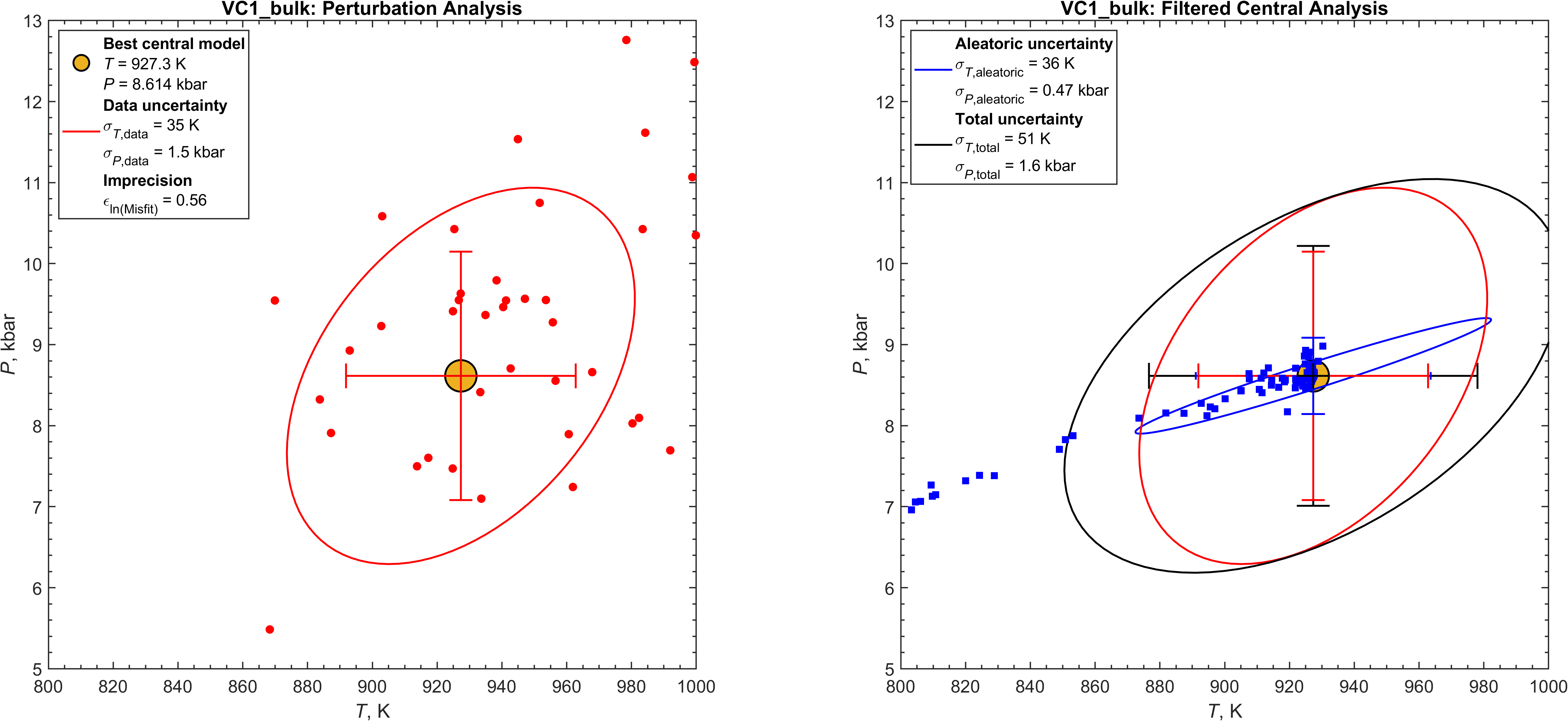
Fig. 12 The VC1_bulk bulk-equilibrium metapelite problem with bulk compositional constraints.
The parallel problem without bulk-compositional constraints is reported in Fig. 17.
When bulk-compositional information is available for bulk-equilibrium problems, both formulations
should be compared. The solution with bulk-compositional constraints is preferred if a phase diagram section is
to be computed. For thermobarometric problems, the solution without bulk-compositional constraints may be preferable.
Uncertainties and correlations involving additional inversion
parameters, in the present case \(\sigma_{C\text{[H2O]}}\) and \(\sigma_{C\text{[O2]}}\), can be
evaluated by selecting the parameters from the mc_fit_plot interface.
Refer to the Fig. 5 and Fig. 8 captions and mc_fit_plot
for additional information on the interpretation of this figure.

Fig. 13 Misfit scatter for the VC1_bulk bulk-equilibrium problem in the \(T \text{-} \ln(\text{misfit})\) plane. Refer to the Fig. 6 and Fig. 9 captions and mc_fit_plot
for additional information on the interpretation of this figure.
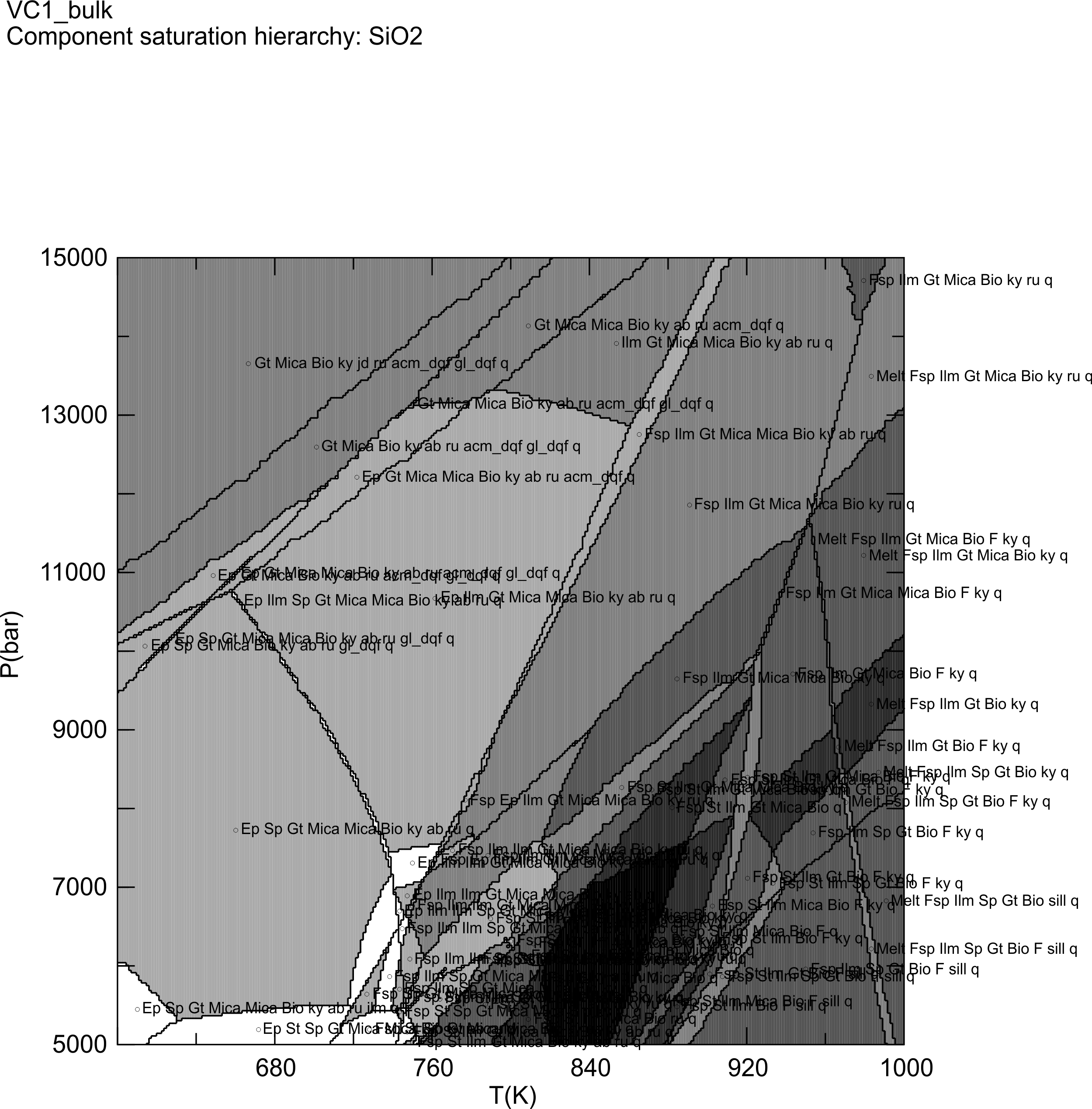
Fig. 14 Phase diagram section computed for the best central model bulk composition obtained by the VC1_bulk inversion (
VC1_bulk.out and
VC1_bulk.dat). The section was computed with vertex and
plotted with pssect.
NOTE: this figure has not been updated to the 7.2.6 mc_fit result.

Fig. 15 Stability field(s) of the observed VC1_bulk garnet + biotite + ilmenite + muscovite + staurolite +
kyanite + quartz assemblage in the section shown in the previous figure. pssect does not discriminate
between multiple phases predicted by a single solution model (e.g., Mica + Mica). The stability fields
of the observed assemblage sensu stricto (Ti-rich Ilmenite,
a single K-rich Mica, +/- Fluid) are the two highest
temperature fields at P = 7000 – 10000 bar.
NOTE: this figure has not been updated to the 7.2.6 mc_fit result.
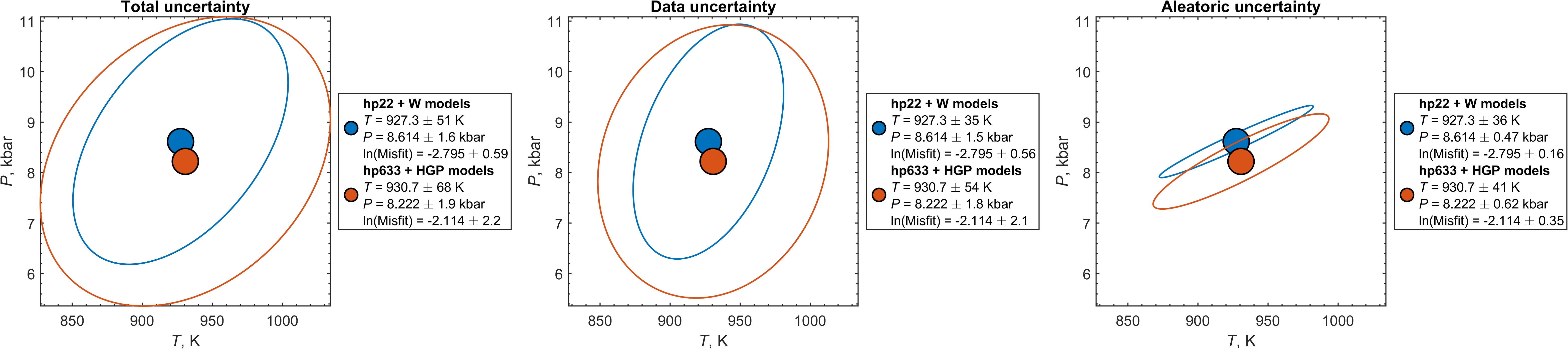
Fig. 16 The VC1_bulk bulk-equilibrium metapelite problem with alternative thermodynamic datasets; hp22 + W models is the reference model, hp633 + HGP models uses the revised Holland et al. 2018 [Holland2018] data and, where
applicable, solution models. Although the differences are not statistically
significant, the reference model dataset yields both a lower misfit and smaller inversion-parameter uncertainties.
The I/O files for this analysis are in VC1_bulk/permutations.
Generated with mc_fit_permutation_plot.
Bulk-equilibrium problems without bulk composition and modal constraints
This category is procedurally identical to local-equilibrium problems. It is presented separately to emphasize that, even in bulk-equilibrium problems for which bulk composition and modal constraints are available, the solution of the thermobarometric inversion problem obtained without the constraints may be preferable or provide insights into the constrained solution. For this reason, it is advisable to first solve the unconstrained inverse problem before adding bulk constraints (see Bulk-equilibrium problems with bulk compositional constraints).
—
VC1_no_bulk: Garnet-zone metapelite unconstrained bulk equilibrium
This problem repeats the VC1_bulk metapelite bulk-equilibrium problem (Fig. 12 and Fig. 13), but without bulk compositional constraints. The resulting thermobarometric estimates are marginally better, both in terms of misfit and uncertainty (Fig. 17 and Fig. 18), although the differences are not statistically significant. The mineral compositions inferred with (Try 302, VC1_bulk.out) and without (Try 281, VC1_no_bulk.out) bulk compositional constraints are remarkably similar, but the bulk composition inferred without bulk compositional constraints is more feldspathic and therefore less water-rich. This result reiterates the point that bulk compositions inferred only from mineral chemistry are not unique and are therefore not an appropriate basis for forward modeling (Appendix B), e.g., to reconstruct the metamorphic history of a rock in a phase diagram section.
The different inferred bulk compositions should not be interpreted as indicating different-quality thermobarometric solutions. Rather, the bulk composition inferred without bulk compositional constraints is one of an infinite number of bulk compositions that are thermodynamically equivalent with respect to the thermobarometric solution.
If modal constraints are available, a bulk composition can be constructed from the corresponding mineral modes in combination with the mineral chemistries predicted by the unconstrained thermobarometric inversion. The resulting bulk composition is a legitimate basis for forward modeling because, by construction, it reproduces the thermobarometric solution.
When measured bulk compositional data are also available, as in the VC1 example, the forward model obtained from the constructed bulk composition can be compared with that obtained from the measured bulk composition. Agreement supports the interpretation that the measured bulk composition is representative of the observed assemblage, whereas disagreement raises questions about the validity of the bulk equilibrium assumption, the measured bulk composition, and/or the thermodynamic data.
—
Additional details:
I/O files: examples/VC1_no_bulk
Chemical system ([Green2016], VC1_no_bulk.dat): Na2O-MgO-Al2O3-SiO2-K2O-CaO-TiO2-MnO-FeO-H2O-O2
Saturated components: SiO2
Unmeasured Components:
component: O2
limit type: coupled
limit expression:
FeO 0 0.0625(\(\text{molar} \left( \frac{\text{Fe}^{3+}}{\text{Fe}^{2+}} \right)_\text{bulk} = \left[0, \frac{1}{3}\right]\), Eq 28)component: H2O
limit type: simple_mass
limit expression:
simple_mass 0 0.0166(\(\text{mass} X_{\text{H2O}} = \left[0, \frac{\text{LOI}}{1 - \text{LOI}}\right]\), LOI = 0.0163, Eq 6)
Data uncertainties:
Analytical (Eq 8, VC1_no_bulk.imc)
Thermodynamic ([Green2016], hp62ver.dat)
Modified Perple_X options (perplex_option.dat): None.
Modified mc_fit options (VC1_MC_fit_option.dat):
number_of_tries and number_of_perturbations increased to
500to ensure adequate sampling of the solution space.
Best central model (Try 281, VC1_no_bulk.out):
\(P\) = 8290.53 bar
\(T\) = 931.860 K
\(C_\text{H2O}\) = 0.201919
\(C_\text{O2}\) = 0.590087
Inversion parameter uncertainties (Fig. 17):
Unmeasured components (Try 281, VC1_no_bulk.out):
\(\text{molar} \left( \frac{\text{Fe}^{3+}}{\text{Fe}^{2+}} \right)_\text{Mu}\) = 0.0223 (Eq 28)
\(\text{molar} \left( \frac{\text{Fe}^{3+}}{\text{Fe}^{2+}} \right)_\text{Gt}\) = 0.00198 (Eq 28)
\(\text{molar} \left( \frac{\text{Fe}^{3+}}{\text{Fe}^{2+}} \right)_\text{Bio}\) = 0.00527 (Eq 28)
\(\text{molar} \left( \frac{\text{Fe}^{3+}}{\text{Fe}^{2+}} \right)_\text{St}\) = 0.00417 (Eq 28)
\(\text{molar} \left( \frac{\text{Fe}^{3+}}{\text{Fe}^{2+}} \right)_\text{Ilm}\) = 0.0307 (Eq 28)
Dependent variables, Oxygen fugacity and Delta QFM (Appendix C):
\(\mu_{\text{O2}}\) = -409983 J/mol (Try 281)
\(\log f_{\text{O2}}\) = -15.091 (bar)
\(\Delta_{\text{QFM}}\) = 2.1961
Bulk composition (Appendix B):
Because this problem employs neither bulk compositional nor modal constraints, the best central model bulk composition (Try 281) is not an appropriate forward model composition for the VC1 rock (see discussion above).
Permutation analysis: see Fig. 19.
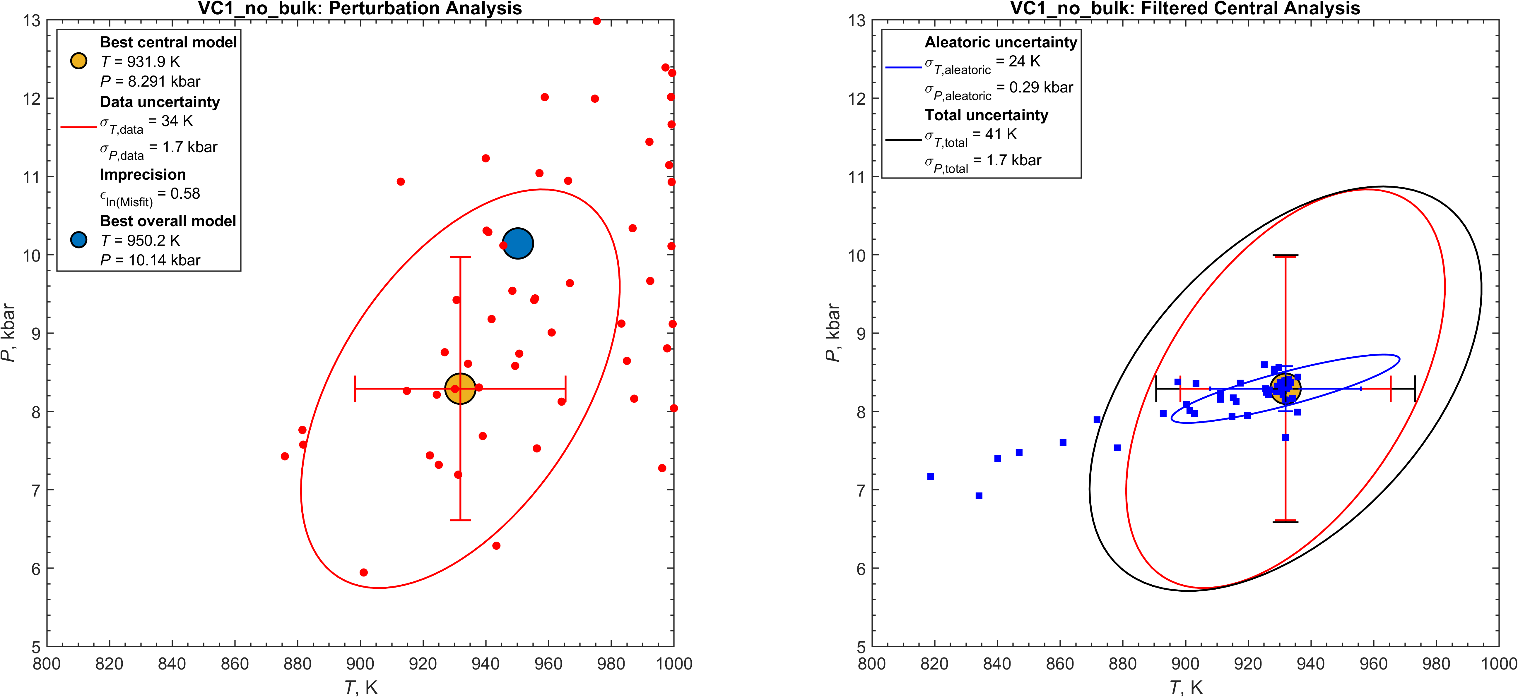
Fig. 17 The VC1_no_bulk problem without bulk compositional constraints.
The parallel problem with bulk compositional constraints is reported in Fig. 12.
When bulk compositional information is available for bulk-equilibrium problems, both formulations
should be compared. The solution with bulk compositional constraints is preferred if a phase diagram section is
to be computed. For thermobarometric problems, the solution without bulk compositional constraints may be preferable.
Uncertainties and correlations involving additional inversion
parameters, in the present case \(\sigma_{C\text{[H2O]}}\) and \(\sigma_{C\text{[O2]}}\), can be
evaluated by selecting the parameters from the mc_fit_plot interface.
Refer to the Fig. 5 and Fig. 8 captions and mc_fit_plot
for additional information on the interpretation of this figure.

Fig. 18 Misfit scatter for the VC1_no_bulk problem in the \(T \text{-} \ln(\text{misfit})\) plane. Refer to the Fig. 6 and Fig. 9 captions and mc_fit_plot
for additional information on the interpretation of this figure.
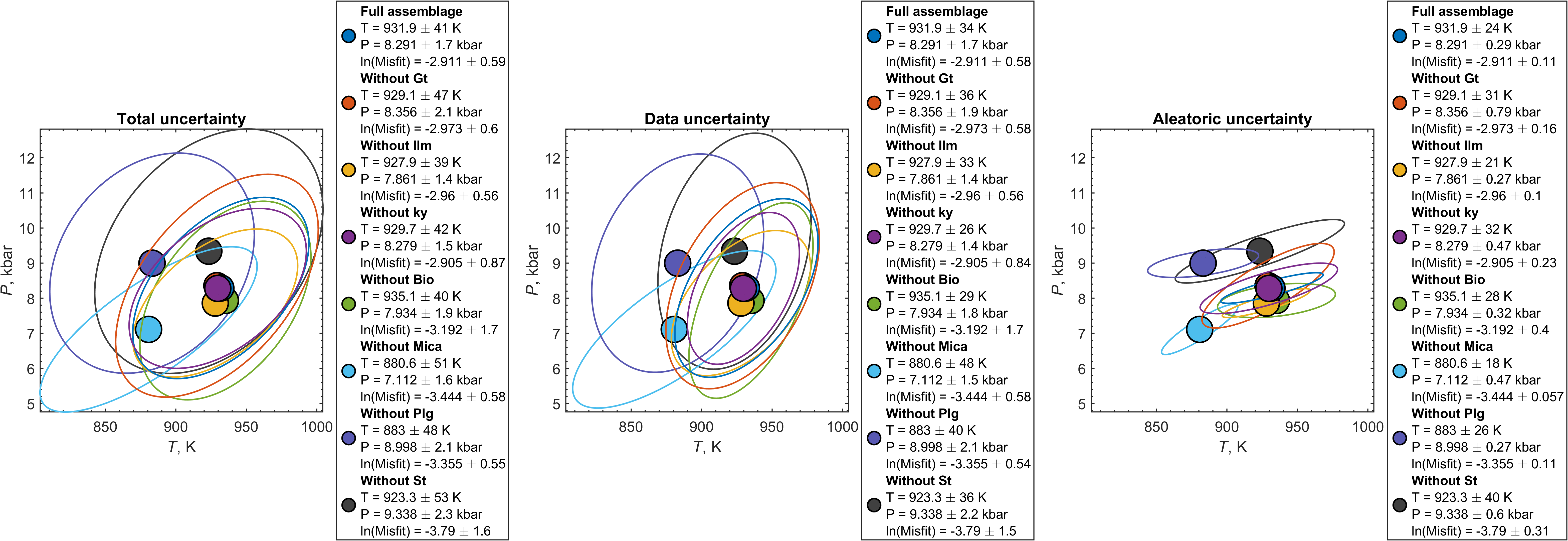
Fig. 19 Comparison of the VC1_no_bulk solution obtained with the full eight-phase assemblage with the solutions for the unique seven-phase permutations of the full assemblage. The covariance ellipses represent 68% coverage (sigma_level = 1); they would be roughly twice as large for the 95% coverage typical of standard statistical analysis.
Thus, at 95% coverage, none of the differences would be statistically significant, supporting the conclusion that the observed assemblage preserves a relict bulk equilibrium. In detail, the largest aleatoric uncertainties are associated with the garnet- and staurolite-absent permutations, suggesting that these phases reduce the ill-conditioning of the inversion problem. In contrast, the three lowest misfit solutions are obtained for the staurolite-, plagioclase-, and muscovite-absent permutations.
Interpretation of these lower misfits is ambiguous because they can be attributed either to inadequacies in the thermodynamic models of the absent phases or to the failure of the absent phases to preserve their equilibrium compositions.
Given the extensive experimental data available for muscovite and plagioclase, and the high diffusive mobility of alkali elements, it is reasonable to conclude that muscovite and plagioclase imperfectly preserve their equilibrium compositions. In contrast, experimental data for staurolite is sparse and it is composed of refractory elements, raising questions about the adequacy of its thermodynamic model.
This interpretation appears at odds with the observation that omission of staurolite increases the aleatoric uncertainty, indicating that staurolite reduces the ill-conditioning of the inversion problem. The apparent contradiction is resolved by recognizing that staurolite constrains the inversion primarily through its restricted stability field, which improves the conditioning of the inversion, whereas its composition governs its contribution to the misfit and is more sensitive to deficiencies in the thermodynamic model.
The I/O files for this analysis are in VC1_no_bulk/permutations. Generated with mc_fit_permutation_plot.
—
Bulk-equilibrium problems with modal constraints
TBD.
