Inversion strategy¶

The mc_fit inversion strategy is implemented by two programs, mc_fit and mc_fit_plot, that together do the inversion parameter optimization and uncertainty analysis. mc_fit identifies the preferred solution and generates the model populations required for uncertainty analysis, whereas mc_fit_plot does statistical analysis of those populations to estimate the uncertainty of the preferred solution.

Throughout the remainder of this chapter, the name mc_fit refers to the methodology except where it is necessary to distinguish the individual programs.

Figures¶

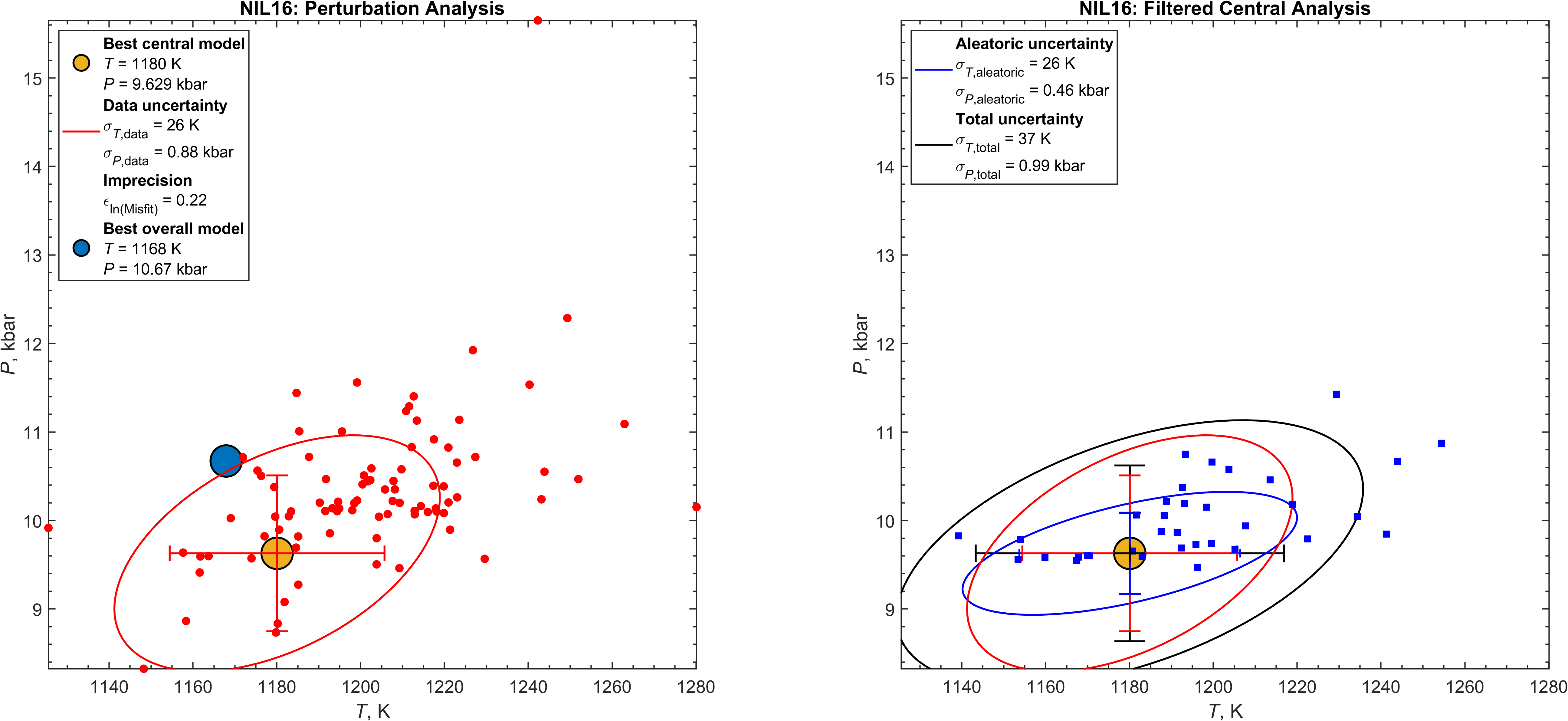
NIL16 garnet + clinopyroxene problem — Fig. 1 Illustration of the uncertainty analysis for an inversion problem (NIL16). **Left panel:** best central model (preferred solution), perturbed model population, and data uncertainty. **Right panel:** filtered central model population and aleatoric and total uncertainties. See Fig. 3 for illustration of the filter.¶

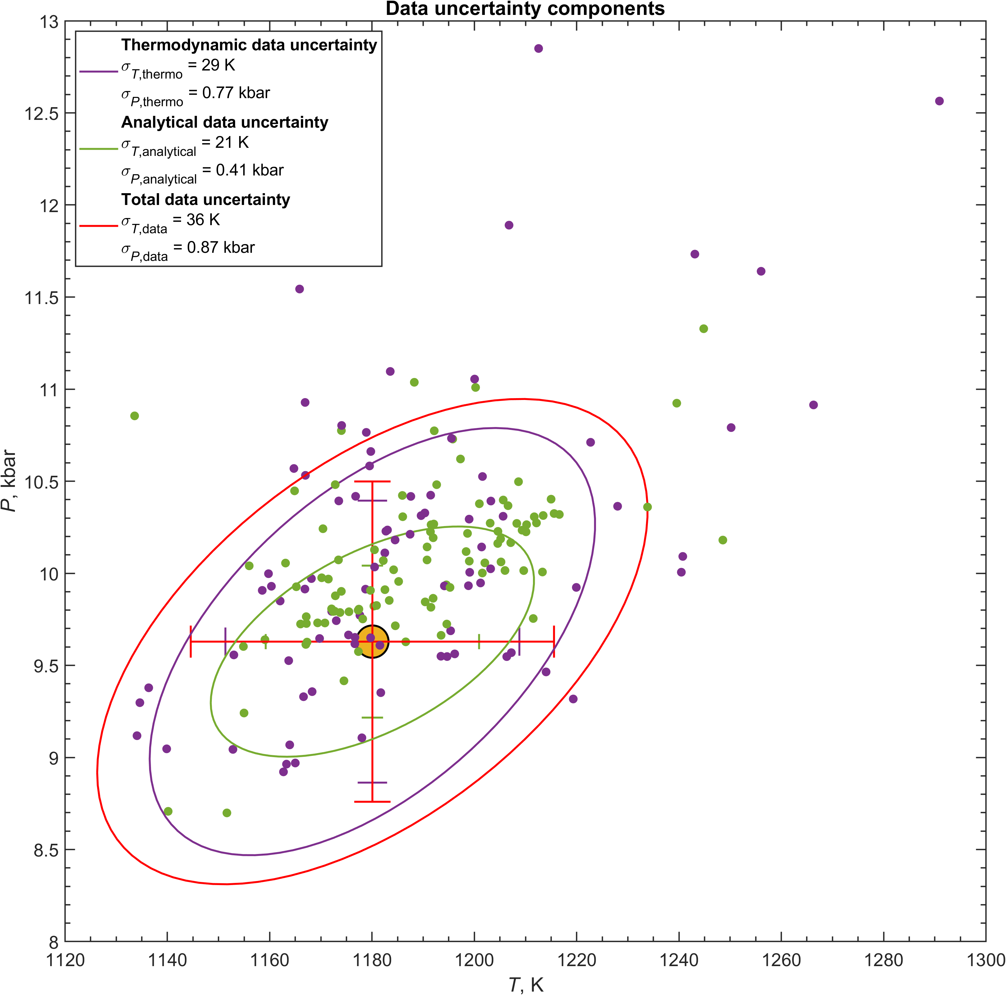
NIL16 data uncertainty components — Fig. 2 Decomposition of the data uncertainty (left panel of Fig. 1) of the NIL16 inversion into its thermodynamic and analytical components.¶

NIL16 imprecision band — Fig. 3 Misfit scatter in the \(T-\ln(\mathrm{misfit})\) plane for the inversion shown in Fig. 1. **Left panel:** the misfit scatter of the perturbed model population defines the misfit imprecision band for the best central model. **Right panel:** central models that lie within the imprecision band are statistically indistinguishable from the best central model. The scatter of these models (right panel of Fig. 1) defines the aleatoric uncertainty of the inverse solution.¶

Inversion parameter optimization¶

Given an initial guess of the inversion parameters and a function that quantifies the misfit between observed and predicted mineralogy, the optimization problem is to find the set of inversion parameters that minimizes this misfit. mc_fit follows Duesterhoef & Lanari ([Duesterhoeft2020], [Khan2021], Slide 7) in using the Nelder-Mead algorithm ([ONeill1971], [MINIM]) to solve the optimization problem.

—

Randomized Nelder-Mead search¶

The Nelder-Mead algorithm is a local minimizer and may miss the global minimum of the misfit function. To mitigate this risk, mc_fit does multiple Nelder-Mead optimizations from randomly generated initial guesses.

This randomized search increases the likelihood of identifying the global minimum of the misfit function (the best-fitting model) and helps assess whether the thermobarometric problem is well-posed. A well-posed problem is characterized by a pronounced global minimum in the misfit function. If the misfit function is flat with respect to an inversion parameter, the problem is ill-posed for that parameter and the solution is not unique.

The goals of the mc_fit optimization strategy are to identify the best-fitting model and the range of models that are statistically indistinguishable given the uncertainty in the input data.

Uncertainty¶

Inversion problems are subject to two sources of uncertainty. Data uncertainty arises from uncertainty in the analytical and thermodynamic data used by the forward model (Fig. 2), whereas aleatoric uncertainty arises from the non-uniqueness of the inverse problem, i.e., multiple solutions may satisfy the data equally well.

Propagation of data uncertainty quantifies both the uncertainty in the inversion parameters (left panel, Fig. 1) and the misfit imprecision, i.e., the uncertainty in the misfit function itself (left panel, Fig. 3). Given the misfit imprecision, it is possible to identify the set of models that are statistically indistinguishable from the preferred solution (right panel, Fig. 3). The scatter of these models characterizes the aleatoric uncertainty of the inverse solution (right panel, Fig. 1). A problem is well-posed when the aleatoric uncertainty is small and ill-posed when it is large.

Central vs. perturbed forward models¶

In mc_fit two types of models are distinguished: central models and perturbed models. Central models are obtained by assigning the observed analytical and thermodynamic data to their central (most probable) values, whereas perturbed models are obtained by perturbing these data within their uncertainty.

Although both central and perturbed models may represent statistically legitimate solutions to the thermobarometric problem, mc_fit adopts the best central model as the preferred solution. Perturbed models are used solely to estimate data uncertainty and misfit imprecision, from which inversion parameter uncertainty is determined, even though some perturbed models may have lower misfit than the best central model.

The rationale for this choice is that the best central model is obtained directly from the observed analytical and published thermodynamic data. In contrast, each perturbed model is specific to a particular realization of the perturbed data. Consequently, subsequent calculations based on a perturbed model would also require the corresponding perturbed data set, whereas the best central model can be reproduced and used directly with the original input data.

Implementation¶

mc_fit implements the inversion strategy in two stages: central model analysis, which identifies the preferred solution; and perturbation analysis, which quantifies data uncertainty and misfit imprecision. The perturbation-derived misfit imprecision is then used to identify the central models that are statistically indistinguishable from the best central model.

—

Central model analysis¶

During the central model analysis, multiple optimizations are done from randomly generated initial guesses of the inversion parameters. Each optimization is referred to as a try. Successful tries generate a population of central models that samples the misfit function over the specified inversion parameter ranges.

The best central model is the central model with the minimum misfit, or the maximum Bayes score when the Bayes option is used. In isolation, the scatter of the central models cannot be interpreted statistically because the precision with which the misfit can be resolved is not known. This deficiency motivates the perturbation analysis which establishes both the misfit imprecision and uncertainty in the inversion parameters attributable to analytical and thermodynamic uncertainties.

—

Perturbation analysis¶

During the perturbation analysis, the analytical and thermodynamic data are randomly perturbed within their uncertainties. For each perturbation, a Nelder-Mead optimization is initiated from the coordinates of the best central model.

The scatter of the perturbed models is used to estimate data uncertainty in the inversion parameters and the misfit imprecision. Because the misfit is strictly positive, its uncertainty is modeled by assuming a log-normal distribution. Accordingly, the misfit imprecision is expressed as the standard deviation of the natural logarithm of the misfit, \(\epsilon_{\ln(\mathrm{misfit})}\).

The central models are then filtered using the misfit imprecision to retain only those whose misfit is statistically indistinguishable from that of the best central model. The scatter of the retained central models characterizes the aleatoric uncertainty of the inverse solution.

For a single inversion parameter \(i\), total uncertainty is obtained by combining data and aleatoric components in quadrature:

(5)¶\[\sigma_{i,\text{total}} = \sqrt{ \sigma_{i,\text{data}}^2 + \sigma_{i,\text{aleatoric}}^2 }\]

where \(\sigma_{i,\text{data}}\) is estimated from the perturbation analysis and \(\sigma_{i,\text{aleatoric}}\) from the retained central models. The corresponding uncertainty intervals are obtained by scaling for the desired coverage probability. The scaling and multi-dimensional analysis used to construct covariance ellipses is summarized in total uncertainty.

Workflow¶

Optimize the inversion parameters using the central analytical and thermodynamic data (mc_fit).
Identify the best central model (mc_fit).
Perturb the analytical and thermodynamic data within their uncertainties (mc_fit).
Estimate data uncertainty and misfit imprecision from the perturbed models (mc_fit_plot).
Use the perturbation-derived misfit imprecision to identify the central models that are statistically indistinguishable from the best central model (mc_fit_plot).
Estimate aleatoric uncertainty from the scatter of the retained central models (mc_fit_plot).
Combine the data and aleatoric components to obtain the total uncertainty (mc_fit_plot).

Note

The logical sequence of the inversion differs from the computational sequence used by mc_fit_plot. mc_fit does the central model analysis before the perturbation analysis. mc_fit_plot processes the perturbation results first because the perturbation-derived misfit imprecision is required to identify the retained central models.

Limitations¶

A consequence of mc_fit’s reliance on the best central model is that successful perturbed models are not reported unless at least one acceptable central model is identified. Thus, in the uncommon circumstance that only perturbed models are successful, mc_fit reports no preferred solution despite the existence of statistically acceptable perturbed solutions.

This limitation reflects the implementation rather than a fundamental restriction. Accommodating such cases would require only minor modifications to the software.